Modeling Fluctuations in the Earth's Magnetic Field
There are a number of parameters that contribute to the fluctuations in earth’s magnetic field. The geomagnetic dipole, or rather its theoretical antipodal points, shift by 0.05 to 0.1 degrees per year, as a result of the flow of molten ferric compounds in the Earth’s crust (Merrill, et al., 1996). More rapid fluctuations in the geosphere can be seen in the actual magnetic North and South dipoles which move independent of one another at rates of up to ∼ 1.27 × 10⁻³ m/s² (Merrill, et al., 1996). These more rapid changes can likely be attributed to the interaction between the interplanetary magnetic field (the IMF), and the region around the Earth in which charged particles are affected by the fields generated by the geomagnetic dipole (i.e., the magnetosphere)—the boundary of the area in space in which these interactions take place is called the magnetopause. The shape and radial distance of the magnetopause is determined by the buffeting by solar winds carrying the IMF, and so the magnetic environment in any region of the Earth differs between day and night phases as the magnetopause compresses the magnetosphere into a bowl-shape under direct pressure from solar winds in the day time, but releases them to stretch out to distances approaching infinity (from our relevant perspective) at night (Van Allen, 2004). Consider that for any position on the surface of the earth, h, there is a point on the magnetosphere, z, that corresponds to the perpendicular distance, DM, from h. Because the density and velocity of solar wind that shape the magnetopause are non-constant along the daytime elevation of the magnetopause, any such effects felt at a particular z₁ resulting in changes to DM1 can be different than those felt at another z₂, and so the corresponding DM2 need not necessarily be the same as DM1. It follows that in the daytime, when DM is effectively finite, z affecting DM must cause fluctuations in the magnitude of δ at h in some way that are regionally specific, that is for two positions, h₁ and h₂, we can expect the magnitude of δʹ₁ to differ nontrivially from that of δʹ₂ over some period Δt if they are separated by some minimum distance Δh (Fig 1). Let us define the region bounded by Δh as H.
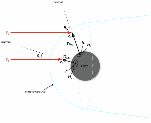
Figure 1. Schematic depicting relationships between points at the surface of the earth, h₁ and h₂, and the corresponding normal vectors, DM1 and DM2, intercept points at the magnetosphere, z₁ and z₂, and solar wind forces p₁ and p₂. Given that the magnetosphere is shaped by the distribution of solar wind forces giving rise to solar wind dynamic pressure, we see that the magnitude of any p determines the magnitude of any DM. Moreover fluctuations in p must give rise to fluctuations in DM. Therefore we can expect that there exists some neighborhood, H₁, around a given point h₁, for which the magnitude of DM1 fluctuates nearly uniformly given a given some distribution of forces around z₁. We can also see that area of H₁ depends in part upon the pressure gradient around z₁, and so the DM1 uniformity cannot extend to some distant neighborhood, H₂, feeling the effects of a pressure gradient around p₂, and where p₂ ≉ p₁. Note too that there exist intrinsic regional affects on the magnitude of DM and how it varies in response to fluctuations in p, which arise from the incident angle θ, and so this contributes to the determination of the area and shape of any H.
As a rudimentary illustration of how δH might be affected by dynamic pressure fluctuations, we can employ the Chapman-Ferraro pressure balance and distance equations (Chapman & Ferraro, 1931):
Where for an arbitrary z: ρsw and Vρsw correspond to the magnitudes of the density and velocity of solar wind, and the angle θ corresponds to the angle of solar wind deflection from the normal. The constant RE is equal to 1 Earth radius, and k ≈ 0.889 (empirically determined). BE, as previously, corresponds to the magnitude of Earth’s magnetic field at the surface, only here we are specifically considering the value at H.
Solving for the magnitude of the solar wind dynamic pressure which we will call psw, in equation (1) gives:
Solving for psw in equation (2) gives
Solving for BE:
From (5) we can derive the following equality:
Substituting this result into (10) gives
Note that
We can therefore write
Since both the solar wind dynamic pressure and magnetopause distance change with time, we can employ the chain rule to define the rate of change of BE:
Recalling that ΔBE(H) = δH, we observe
which expresses δʹ in region H, changing with specificity as a function of the solar wind dynamic pressure at z. This is theoretically solvable as a constant rate, and so can be theoretically used in the derivation of Λ in equation (43) of part one of this model, Modeling Genomic Fixation Probabilities of Tautomeric Mutations as a Function of Characteristic Fluctuations in Earth’s Magnetic Field.
This model suggests a trend of increasing mutation potential (and with it genomic diversity) as region H approaches the equator, and this is consistent with current literature (Meyers, et al., 2000). The object of this speculative two-part model is to argue the existence of relationships between the parameters involved, rather than to provide rigorous explanations of such relationships—which would necessitate a comprehensive handling of the R entities in part one, a more modern handling of the modeling in part two, and, of course experimentation. Therefore the value of the models is in the corollaries and hypotheses they give rise to. I leave it to the reader to explore these implications.